Python - Detect outliers using moving average

In this piece of code, you can change window_size to determine how you want to calculate the average. e.g. using 6 months of adjacent data. You can change the sigma_value to determine the abnormal points you want to capture. e.g. if you assume 99.7% of data are normally distributed, then set sigma_value= 3. You can change the start and end values to determined how many months of production you want to see.

from scrapers import config_sql
from itertools import count
import matplotlib.pyplot as plt
import numpy as np
import pandas as pd
import collections


def moving_average(data, window_size):
    weight = np.ones(int(window_size)) / float(window_size)
    return np.convolve(data, weight, 'same')  # ways to handle edges. the mode are 'same', 'full', 'valid'


def detect_anomalies(y, window_size, sigma):
    # slide a window along the input and compute the mean of the window's contents
    avg = moving_average(y, window_size).tolist()
    residual = y - avg
    # Calculate the variation in the distribution of the residual
    std = np.std(residual)
    return {'standard_deviation': round(std, 3),
            'anomalies_dict': collections.OrderedDict([(index, y_i) for index, y_i, avg_i in zip(count(), y, avg) if (y_i > avg_i + (sigma * std)) | (y_i < avg_i - (sigma * std))])}  # distance from the mean


# This function is responsible for displaying how the function performs on the given dataset.
def plot_results(x, y, window_size, sigma_value, text_xlabel, text_ylabel, start, end):
    plt.figure(figsize=(15, 8))
    plt.plot(x, y, "k.")
    y_av = moving_average(y, window_size)
    try:
        plt.plot(x, y_av, color='blue')
        plt.plot(x, y, color='green')
        plt.xlim(start, end)  # this can let you change the plotted date frame
        plt.xlabel(text_xlabel)
        plt.ylabel(text_ylabel)

        events = detect_anomalies(y, window_size=window_size, sigma=sigma_value)
        x_anomaly = np.fromiter(events['anomalies_dict'].keys(), dtype=int, count=len(events['anomalies_dict']))
        y_anomaly = np.fromiter(events['anomalies_dict'].values(), dtype=float, count=len(events['anomalies_dict']))
        print(collections.OrderedDict([(x, y) for index, x, y in zip(count(), x_anomaly, y_anomaly)]))
        ax = plt.plot(x_anomaly, y_anomaly, "r.", markersize=12)

        # add grid and lines and enable the plot
        plt.grid(True)
        plt.show()

    except Exception as e:
        pass

# Main
if __name__ == '__main__':
    conn = config_sql.sql_credentials('XXXXX', 'XXXX')
    cursor = conn.cursor()

    query = "XX where bridge_Id in('8368051','8502207','8369707','8520772','8420250','12776634')"

    df = pd.read_sql(query, conn)
    cols = ['bridge_id', 'product_name', 'metric_date', 'prod_value']
    oil_prod = df.loc[df['product_name'] == 'Gas']
    prod_as_frame = pd.DataFrame(oil_prod, columns=['bridge_id', 'product_name', 'metric_date', 'prod_value'])

    # get unique list of bridge
    rows = cursor.execute(query)
    unique_bridge = set(list(zip(*list(rows.fetchall())))[0])

    for bridge_id in unique_bridge:
        print('bridge_Id: ' + str(bridge_id))
        prod = prod_as_frame[prod_as_frame.bridge_id == bridge_id].reindex()
        prod['mop'] = range(1, len(prod) + 1)

        x = prod['mop']
        Y = prod['prod_value']
        max_x = max(x) # this can let you change the plotted date frame
        print(prod)

        # plot the results
        plot_results(x, y=Y, window_size=6, sigma_value=3, text_xlabel="MOP", text_ylabel="production", start=1, end=max_x)

Background knowlodge:

np.std

To quantify the amount of variation or dispersion of dataset.
Low std means data points tend to be close to the mean; high std means the data points are spread out over a wide range of values.
np.Convolve

Is defined as the integral of the product of two functions after one is reversed and shifted.
It is an operation on two functions to produce a third function that express how the shape of one is modified by the other.
Rules of normally distributed data (68-95-99.7 rule)

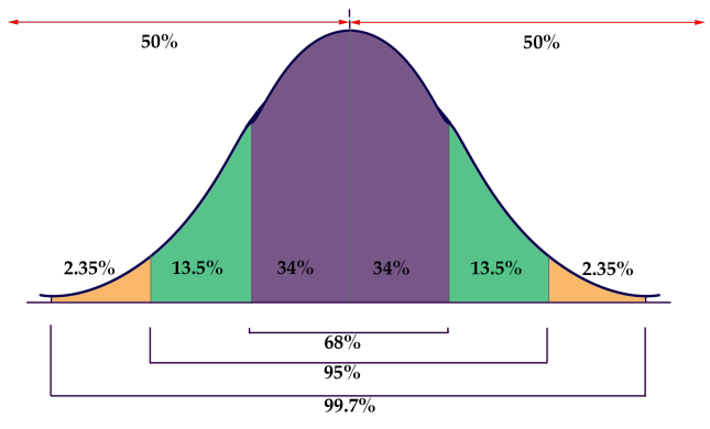
If a data distribution is approximately normal, then about 68% of the data value are within 1 std of the mean