Python - Return the indexes of all occurrences of a string in a list

Here is the function to return the indexes of a certain string occurrences in a list:

def getIndexPositions(listOfString, certainString):
    ''' Returns the indexes of all occurrences of give element in    

        the list- listOfString'''

    indexList = []
    indexPos = 0    

    while True:
        try:
            # Search for item in list from indexPos to the end of list            

            indexPos = listOfString.index(certainString, indexPos)
            # Add the index position in list            

            indexList.append(indexPos)
            indexPos += 1        

        except ValueError as e:
            break
    return indexList

SQL - search for column/table name in database

USE the database you want to search;
SELECT      c.name  AS 'ColumnName' ,t.name AS 'TableName'
FROM        sys.columns c  JOIN sys.tables  t ON c.object_id = t.object_id
WHERE       (t.name like 'LA%' or t.name like '%luw%' or t.name like 'Louisana%' )
        and c.name in ('API','API_NUM','API num','Well_Serial_Num','Well_Serial_No','WELL_SERIA','Well Serial Number','WSN','Serial_no','Well_Serial','well Serial Num')
ORDER BY    TableName  ,ColumnName;

Python - some tricks with web scrapping ( decompose(), zip(), modify html tags, etc.)

• If there are some junk html tab within the tab you want to scrape, e.g.

<table align="center" border="0" cellpadding="0" cellspacing="0" height="0%" summary="Scout Ticket well data content table" width="98%">
......data you want to scrape.......
<table border="0" cellpadding="0" cellspacing="0" height="0%" summary="Plan View Table" width="100%">....junk table....</table>
-----data you want to scrape
</table>

then you can use:  soup.decompose()

for table_useless in soup.find_all("table", {"summary": "Plan View Table"}):
    table_useless.decompose()

• If there are tags within another tag, you can extract data separately and zip them together, e.g.

<td>NDIC File No: <b>12584</b></td>, <td>     API No: <b>33-007-01163-00-00</b></td>

then you can use: zip()

header_data = [html.get_contents(header.next) for header in data_points]

detail_data = [item.find('b').next if item.find('b') is not None else 'None' for item in data_points]

final_data = dict(zip(header_data, detail_data))

Python - function to convert .csv file to multiple .json files

This function was used in QA process, when I have one input of .csv file, and I want to test each individual row of data
.
This is production.csv file:

api,prod_date,oil,water,cond,gas
42003024530000,2014-04-01,22,34,0,4928
42003024530000,2014-05-01,30,334,0,4328
42003024530000,2014-06-01,20,44,0,2228
42003024530000,2014-07-01,20,164,0,3328
42003024530000,2014-08-01,0,164,46,3600

This is how data looks like when written into individual json file:

[{

    "api": "42003024530000",

    "prod_date": "2014-04-01",

    "oil": "22",

    "water": "34",

    "cond": "0",

    "gas": "4928"

}]

# Convert csv data into jsondef convert_write_json(data, json_file_name, directory):
    with open(os.path.join(current_directory, 'TestData', directory, json_file_name + '.json'), "w") as f:
        f.write('[' + json.dumps(data, sort_keys=False, indent=4, separators=(',', ': ')) + ']')

Method 1: right file into a single json file

# Read CSV File and write into a single json filedef read_production_csv(csv_file_name, json_file, directory):
    for item in directory:
        csv_rows = []
        csv_file_path = os.path.join(current_directory, 'TestData', csv_file_name + '.csv')
        with open(csv_file_path) as csv_file:
            reader = csv.DictReader(csv_file)
            field = reader.fieldnames
            for row in reader:
                csv_rows.extend([{field[i]:row[field[i]] for i in range(len(field))}])
            convert_write_json(csv_rows, json_file, item)

Method 2: right each row in the file into a separate json file

# Read CSV File and write each row into a separate json file

def read_production_csv(csv_file_name, directory):
    for item in directory:
        csv_file_path = os.path.join(current_directory, 'TestData', csv_file_name + '.csv')
        with open(csv_file_path) as csv_file:
            reader = csv.DictReader(csv_file)
            for row in reader:
                api = row['api']
                prod_date = row['prod_date']
                json_file_name = 'production_' + api + '_' + prod_date
                convert_write_json(row, json_file_name, item)

SQL - LEAD and LAG functions to calculate differences between different rows

Reference:
https://www.mssqltips.com/sqlservertutorial/9127/sql-server-window-functions-lead-and-lag/

Usage in industry:

For example, you have a lot of data from directional survey, and you have data measured depth, and inclination. You would like to know the first inclination point which turns or greater than 80, since that might be the place where the well becomes directional. And the length till that point would be vertical depth, total measured depth - depth till that point is lateral length. But you need to check the distance between that point (in my example P2) and its previous point (P1) to make sure that the distance is less that 200, then that confirms the data is right (at least the percentage of data accuracy is high). In this case, you can use Lag() function.

So, by using lag() function, you can do:

select api, max_MD,Lag(DS_MD,1) OVER(PARTITION BY api ORDER BY DS_MD) as previous_VD
from.....

SQL - Pivot row values as column names in select statement (Concatenate row values)

QUOTENAME()

Return a Unicode string with bracket delimiters (default):

or SELECT QUOTENAME('abcdef', '()') returns (abcedf)

FOR XML PATH(''), TYPE

converts these rows into a single strongly-typed XML text node with the concatenated rows.

Adding FOR XML PATH to the end of a query allows you to output the results of the query as XML elements, with the element name contained in the PATH argument. For example, if we were to run the following statement:

SELECT ',' + name 
              FROM temp1
              FOR XML PATH ('')

By passing in a blank string (FOR XML PATH('')), we get the following instead:

,aaa,bbb,ccc,ddd,eee

Invoking the method value('.', 'NVARCHAR(MAX)') on that XML node converts the XML node to an nvarchar(MAX) string. 

STUFF()

Remove leading comma with STUFF.

The STUFF statement literally "stuffs” one string into another, replacing characters within the first string. We, however, are using it simply to remove the first character of the resultant list of values.

SELECT abc = STUFF((
            SELECT ',' + NAME
            FROM temp1
            FOR XML PATH('')
            ), 1, 1, '')
FROM temp1

So we end up with:

aaa,bbb,ccc,ddd,eee

Example:

IF OBJECT_ID('dbo.tbl_XXXX','U') IS NOT NULL DROP TABLE dbo.tbl_tbl_XXXX

DECLARE @cols AS NVARCHAR(MAX),@query AS NVARCHAR(MAX) ; SET @cols = STUFF(( SELECT ',' + QUOTENAME(data_refresh_date) FROM dbo.tbl_some_source GROUP BY data_refresh_date order by data_refresh_date FOR XML PATH(''), TYPE).value('.', 'NVARCHAR(MAX)'),1,1,'')

set @query = 'SELECT state,Play,attribute, metric_level,' + @cols + ' from ( SELECT DISTINCT A.state,A.Play,A.attribute,A.metric_level, A.data_refresh_date,

CONVERT(varchar,A.cnt*100/B.cnt,2) + ''%'' perc

FROM dbo.tbl_some_source A INNER JOIN dbo.tbl_some_source B ON A.State = B.State AND A.Play = B.play AND B.data_refresh_date = A.data_refresh_date AND B.attribute = ''API_Count'' ) x pivot ( max(perc) for data_refresh_date in (' + @cols + ') ) p '

execute('SELECT * INTO dbo.tbl_destination FROM (' + @query + ')x')

Explanation:

The xml part returns an xml result as:

Then by using dynamic SQL, we can use the result as column names to pivot data:

Other reference:

https://www.red-gate.com/simple-talk/sql/t-sql-programming/concatenating-row-values-in-transact-sql/

Python - Detect outliers using moving average

In this piece of code, you can change window_size to determine how you want to calculate the average. e.g. using 6 months of adjacent data. You can change the sigma_value to determine the abnormal points you want to capture. e.g. if you assume 99.7% of data are normally distributed, then set sigma_value= 3. You can change the start and end values to determined how many months of production you want to see.

from scrapers import config_sql
from itertools import count
import matplotlib.pyplot as plt
import numpy as np
import pandas as pd
import collections


def moving_average(data, window_size):
    weight = np.ones(int(window_size)) / float(window_size)
    return np.convolve(data, weight, 'same')  # ways to handle edges. the mode are 'same', 'full', 'valid'


def detect_anomalies(y, window_size, sigma):
    # slide a window along the input and compute the mean of the window's contents
    avg = moving_average(y, window_size).tolist()
    residual = y - avg
    # Calculate the variation in the distribution of the residual
    std = np.std(residual)
    return {'standard_deviation': round(std, 3),
            'anomalies_dict': collections.OrderedDict([(index, y_i) for index, y_i, avg_i in zip(count(), y, avg) if (y_i > avg_i + (sigma * std)) | (y_i < avg_i - (sigma * std))])}  # distance from the mean


# This function is responsible for displaying how the function performs on the given dataset.
def plot_results(x, y, window_size, sigma_value, text_xlabel, text_ylabel, start, end):
    plt.figure(figsize=(15, 8))
    plt.plot(x, y, "k.")
    y_av = moving_average(y, window_size)
    try:
        plt.plot(x, y_av, color='blue')
        plt.plot(x, y, color='green')
        plt.xlim(start, end)  # this can let you change the plotted date frame
        plt.xlabel(text_xlabel)
        plt.ylabel(text_ylabel)

        events = detect_anomalies(y, window_size=window_size, sigma=sigma_value)
        x_anomaly = np.fromiter(events['anomalies_dict'].keys(), dtype=int, count=len(events['anomalies_dict']))
        y_anomaly = np.fromiter(events['anomalies_dict'].values(), dtype=float, count=len(events['anomalies_dict']))
        print(collections.OrderedDict([(x, y) for index, x, y in zip(count(), x_anomaly, y_anomaly)]))
        ax = plt.plot(x_anomaly, y_anomaly, "r.", markersize=12)

        # add grid and lines and enable the plot
        plt.grid(True)
        plt.show()

    except Exception as e:
        pass

# Main
if __name__ == '__main__':
    conn = config_sql.sql_credentials('XXXXX', 'XXXX')
    cursor = conn.cursor()

    query = "XX where bridge_Id in('8368051','8502207','8369707','8520772','8420250','12776634')"

    df = pd.read_sql(query, conn)
    cols = ['bridge_id', 'product_name', 'metric_date', 'prod_value']
    oil_prod = df.loc[df['product_name'] == 'Gas']
    prod_as_frame = pd.DataFrame(oil_prod, columns=['bridge_id', 'product_name', 'metric_date', 'prod_value'])

    # get unique list of bridge
    rows = cursor.execute(query)
    unique_bridge = set(list(zip(*list(rows.fetchall())))[0])

    for bridge_id in unique_bridge:
        print('bridge_Id: ' + str(bridge_id))
        prod = prod_as_frame[prod_as_frame.bridge_id == bridge_id].reindex()
        prod['mop'] = range(1, len(prod) + 1)

        x = prod['mop']
        Y = prod['prod_value']
        max_x = max(x) # this can let you change the plotted date frame
        print(prod)

        # plot the results
        plot_results(x, y=Y, window_size=6, sigma_value=3, text_xlabel="MOP", text_ylabel="production", start=1, end=max_x)

Background knowlodge:

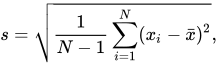
np.std

To quantify the amount of variation or dispersion of dataset.
Low std means data points tend to be close to the mean; high std means the data points are spread out over a wide range of values.
np.Convolve

Is defined as the integral of the product of two functions after one is reversed and shifted.
It is an operation on two functions to produce a third function that express how the shape of one is modified by the other.
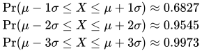
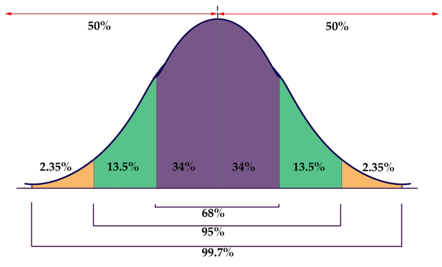
Rules of normally distributed data (68-95-99.7 rule)

If a data distribution is approximately normal, then about 68% of the data value are within 1 std of the mean